- Part I: Non-linear dispersive PDE with boundary ?
- Context & Notations
- Modelisation of the problem
- Part II: Some theory
- Reformulation of the problem as a boundary problem
- Well-posedness of the problem
- Part III: Numerical point of view
- Numerical simulations
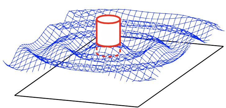
Context
- Axisymetry with respect to the axis of revolution of the cylinder,
- Conservation of irrotationnality,
- The fluid fits the bottom of the cylinder under the cylinder.
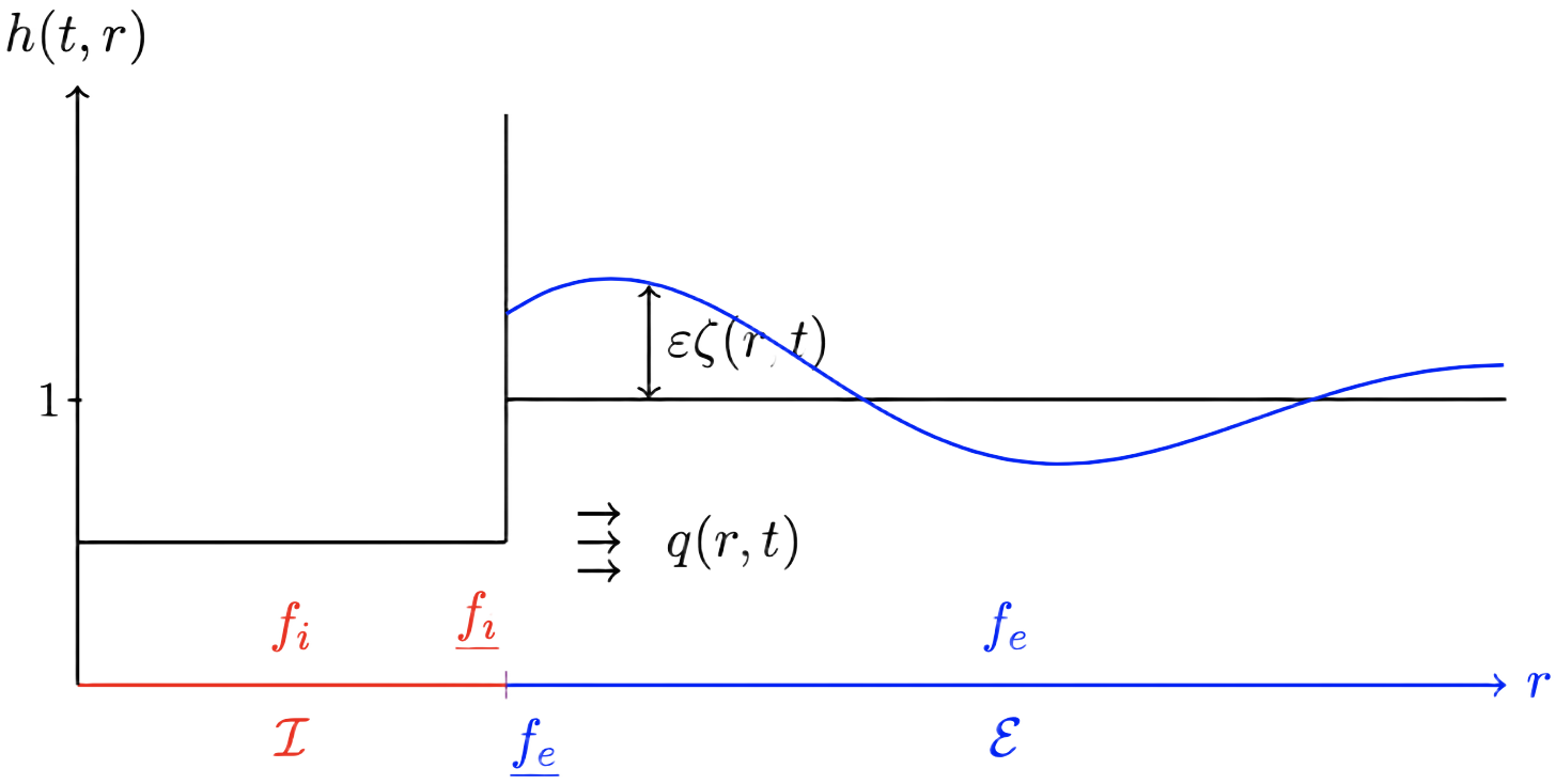
Notations
-
$\varepsilon = \frac{\text{typ. wave amplit.}}{\text{typ. depth}}$; $\kappa = \frac{\text{typ. depth}}{\text{typ. horiz. scale}}$
-
$\zeta$ - Elevation of the wave
-
$h = 1 + \varepsilon \zeta$ - Height of the water
-
$q = hu$ - Discharge
-
$\delta$ - Position of the solid
-
$P$ - Pressure at the surface
Remarks:
- In $\mathcal{I}, \dot{\zeta}_i = \dot{\delta}$ and $P_i$ is unknown
- In $\mathcal{E}, P_e = P_{atm}$ and $\zeta_e$ is unknown
Boussinesq-Abbott equations:
$$ \left\{\begin{matrix} \partial_t \zeta + {\rm div}q = 0, \\ (1-\class{fragment highlight-blue}{\kappa^2 \partial_r {\rm div}})\partial_t q + \class{fragment highlight-blue}{\varepsilon {\rm div} \frac{q^2}{h}+ h\partial_r \zeta} = - h \partial_r P, \\ h = 1 + \varepsilon \zeta. \end{matrix}\right. $$
-
A very (maybe) last notation:
- $\underline{f_e} = \underset{\rho \to R}{\lim}f(r+\rho)$
-
Transmission conditions:
- $\underline{q_i} = \underline{q_e}$
- $\underline{P_i} = \mathcal{L}(\zeta, q, \delta)$
-
Remark:
- Since $\dot{\zeta}_i = \dot{\delta}$, then $\underline{q_e} = -\frac{R}{2}\dot{\delta}$
Theorem 1 Reformulation
$$ \left\{\begin{matrix} \partial_t \zeta + {\rm div}q = 0, \\ (1-\kappa^2 \partial_r {\rm div})\partial_t q + \varepsilon {\rm div} \frac{q^2}{h}+ h\partial_r \zeta = - h \partial_r P, \\ h = 1 + \varepsilon \zeta, \end{matrix}\right. \quad r \geq 0, \, t > 0.$$
$$ \left\{\begin{matrix} \partial_t \zeta + \partial_r q = -\frac{q}{r}, \\ \partial_t q + \partial_r \mathcal{F}_\kappa[\zeta, q] = -\ddot{\delta} K(r/\kappa), \\ \underline{q} = -R\dot{\delta}, \end{matrix}\right. \quad r > R, \, t > 0 \quad + \quad \left\{\begin{matrix} \kappa^2\ddot{\zeta} + \zeta = \mathcal{F}(\zeta) - G\ddot{\delta} + \varepsilon \mathcal{N}(\zeta, q, \underline{\zeta}, \delta), \\ \tilde{m} \ddot{\delta} + \delta + \varepsilon a(\delta) \dot{\delta}^2 = \kappa^2\ddot{\underline{\zeta}} + \underline{\zeta} + \mathcal{F}(\zeta), \end{matrix}\right. \quad t > 0. $$
- Reformulation of the Newton's equation
-
Inversion of the dispersive operator $(1-\kappa^2 \partial_r {\rm div})$:
-
Operators $\mathfrak{R}_0$ & $\mathfrak{R}_1$ defined as:
$$ \forall f, \mathfrak{R}_0 f = f \Leftrightarrow \left\{\begin{matrix} (1-\kappa^2 \partial_r {\rm div})\mathfrak{R}_0 f = f \\ \underline{\mathfrak{R}_0 f} = 0 \end{matrix}\right., \quad \mathfrak{R}_1 f = f \Leftrightarrow \left\{\begin{matrix} (1-\kappa^2 {\rm div}\partial_r)\mathfrak{R}_1 f = f \\ \underline{\partial_r\mathfrak{R}_1 f} = 0 \end{matrix}\right. $$
- Commutation formula: $$\mathfrak{R}_0\partial_r = \partial_r \mathfrak{R}_0.$$
- Bounded operators on $L^\infty$ and $L^2$: if $u \in L^\infty$ (resp $u \in L^2$) then $\mathfrak{R}_{i}u \in L^\infty$ (resp $\mathfrak{R}_{i}u \in L^2$)
-
Operators $\mathfrak{R}_0$ & $\mathfrak{R}_1$ defined as:
- Application of $\kappa^2{\rm div}$, use $\partial_t\zeta = - {\rm div}q$ and take the result in $r = R$
$$ \class{fragment highlight-blue}{(m + \kappa^2 + \frac{R^2}{8})\ddot{\delta} + \delta = \kappa^2 \underline{\ddot{\zeta}} + \underline{\zeta}.} $$
Definition Well-posedness
Definition The space $H^1_r$
Theorem 2 Well-posedness of the Augmented formula
For a general PDE of unknown $u$ with initial condition $u_0$ under the form $$ \partial_t u + Au = \mathcal{F}, $$
the formal solution is given by the Duhamel's formula: $$ \forall t > 0, t < T^*, \, u(t) = e^{tA}u_0 + \underset{\text{Contractant ?}}{\underbrace{\int_0^t e^{(t-s)A}\mathcal{F}(s)ds}}. $$
Goal: for a nonlinear PDE, obtaining a contractant estimate for $\mathcal{F} \class{fragment}{= \mathcal{F}[u]}$
-
$$ \left\{\begin{matrix} \partial_t u + \partial_r \mathfrak{F}_\kappa [u, Z] = \varepsilon \mathcal{F}[u, Z], \\ \partial_t Z + \mathfrak{G}(u, Z) = \varepsilon \mathcal{G}(u, Z). \end{matrix}\right. $$$$ \left\{\begin{matrix} \partial_t u^{k+1} + \partial_r \mathfrak{F}_\kappa [u^{k+1}] = \varepsilon \mathcal{F}[u^k, Z^k],\\ \partial_t Z^{k+1} + \mathfrak{G}(u^{k+1}, Z^{k+1}) = \varepsilon \mathcal{G}(u^{k}, Z^{k}). \end{matrix}\right. $$
- Goal: for $u_1, u_2$, $Z_1, Z_2$, control of type $$ ||\mathcal{F}[u_1, Z_1](t) - \mathcal{F}[u_2, Z_2](t)||_{Y} \leq C t||(u_1, Z_1) - (u_2, Z_2)||_{X} $$ and $$ |\mathcal{G}[u_1, Z_1](t) - \mathcal{G}[u_2, Z_2](t)| \leq \tilde{C} t||(u_1, Z_1) - (u_2, Z_2)||_{X} $$ for $C, \tilde{C} > 0$ independant of $t$.
- In this case the nonlinearities are contractant while $t < \max(C^{-1}, \tilde{C}^{-1})$.
Theorem 3
- Computation of $\mathfrak{R}_1 \zeta$
- Computation of $\delta$ and $\zeta$
- Reconstruction of $q$ (Optionnal)
- Discretization of $\mathfrak{R}_1$ as an elliptic problem,
- Space's discretization not truely important,
- CFL of the form: $$\Delta t \lesssim \kappa \quad \& \quad \Delta x \lesssim \kappa.$$
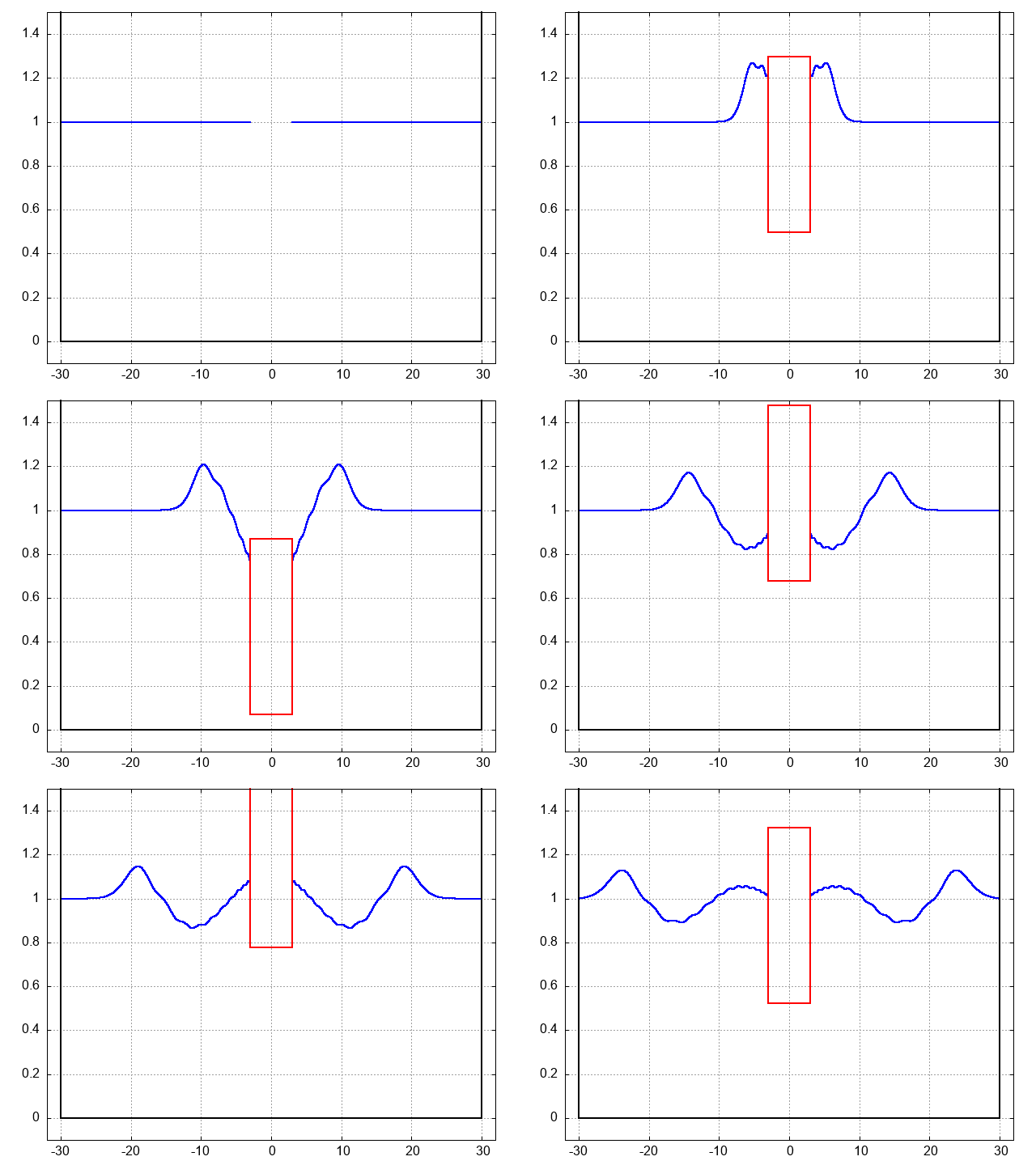
Figure - Simulation
- Well-posedness with time existence uniform in $\kappa$ in order to obtain the shallow-water asymptotic,
- Well-posedness with a larger time existence in the linear case,
- A spectral scheme for the small values of $\kappa$,
- Non-linear case for the numerical analysis,
- Flux scheme for the numerical simulations,
- Model without the symetries.
- Later again: Ice sheet model to understand the ice sheet fracturation.
Thank you!
Slides created using reveal.js
