Part I: Modelisation of the problem
Context & Notations
Modelisation & Reformulation of the problem
Part II: A first scheme for the numerical simulations
Discretization
Energy inequalities
Part III: Shallow-water asymptotic & spectral scheme
Spectral scheme
Comparison with the first method
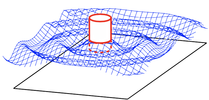
Figure - Freely floating cylinder
Context
Cylinder of radius $R > 0$,
Axisymetry with respect to the axis of revolution of the cylinder,
Conservation of irrotationnality,
The fluid fits the bottom of the cylinder under the cylinder,
Case of the return to the equilibrium.
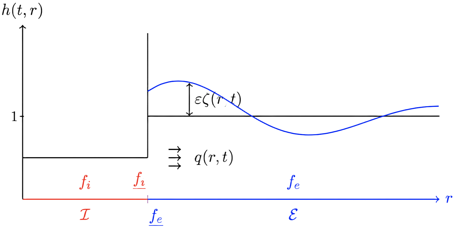
Figure - Slice of the problem
Notations
$\kappa = \frac{\text{typ. depth}}{\text{typ. horiz. scale}}$
$\zeta$ - Elevation of the wave
$h = h_{\rm eq} + \zeta$ - Height of the water
$q = hu$ - Discharge
$\delta$ - Position of the solid
$P$ - Pressure at the surface
Remarks:
In $\mathcal{I}, \dot{\zeta}_i = \dot{\delta}$ and $P_i$ is unknown
In $\mathcal{E}, P_e = P_{atm}$ and $\zeta_e$ is unknown
Boussinesq-Abbott equations:
$$ \left\{\begin{matrix}
\partial_t \zeta + {\rm d}_r q = 0, \\
(1-\kappa^2 \partial_r {\rm d}_r)\partial_t q +
\partial_r \zeta
= - \partial_r P, \\
{\rm d}_r = \partial_r + \frac{d-1}{r}.
\end{matrix}\right. $$
Newton's equation:
$$m\ddot{\delta} + mg = \int_\mathcal{I} P$$
A very (maybe) last notation:
$\underline{f_e} = \underset{\rho \to R}{\lim}f(r+\rho)$
Transmission conditions:
$\underline{q_i} = \underline{q_e}$
$\underline{P_i} = \mathcal{L}(\zeta, q, \delta)$
Remark:
Since $\dot{\zeta}_i = \dot{\delta}$, then $\underline{q_e} = -\frac{R}{2}\dot{\delta}$
Theorem 1
Reformulation
PDE system on $\mathbb{R}^+$ + Transmission conditions
$$ \left\{\begin{matrix}
\partial_t \zeta + {\rm d}_r q = 0, \\
(1-\kappa^2 \partial_r {\rm d}_r)\partial_t q + \partial_r \zeta = - \partial_r P, \\
\end{matrix}\right. \quad r \geq 0, \, t > 0.$$
$$ \Updownarrow $$
Augmented formula : PDE system on $(R, +\infty)$ + ODE at the boundary
$$ \left\{\begin{matrix}
\partial_t \zeta + \partial_r q = -\frac{q}{r}, \\
\partial_t q + \partial_r \mathcal{R}\zeta = -\ddot{\delta} K(r/\kappa), \\
\underline{q} = -R\dot{\delta},
\end{matrix}\right. \quad r > R, \, t > 0 \quad + \quad \left\{\begin{matrix}
\kappa^2\underline{\ddot{\zeta}} + \underline{\zeta} = \underline{\mathcal{R}\zeta} - G(R/\kappa)\ddot{\delta}, \\
\tilde{m} \ddot{\delta} + \delta = \kappa^2\ddot{\underline{\zeta}} + \underline{\zeta},
\end{matrix}\right. \quad t > 0. $$
$$ \left\{\begin{matrix}
\partial_t \zeta + {\rm d}_r q = 0, \\
(1-\kappa^2 \partial_r {\rm d}_r)\partial_t q + \partial_r \zeta = 0,
\end{matrix}\right. \quad r > R.$$
Reformulation of the Newton's equation
Inversion of the dispersive operator $(1-\kappa^2 \partial_r {\rm d}_r)$:
Operators $\mathfrak{R}_0$ & $\mathfrak{R}_1$ defined as:
$$
\forall f, \mathfrak{R}_0 f = f \Leftrightarrow \left\{\begin{matrix} (1-\kappa^2 \partial_r {\rm d}_r)\mathfrak{R}_0 f = f \\ \underline{\mathfrak{R}_0 f} = 0 \end{matrix}\right.,
\quad
\mathfrak{R}_1 f = f \Leftrightarrow \left\{\begin{matrix} (1-\kappa^2 {\rm d}_r\partial_r)\mathfrak{R}_1 f = f \\ \underline{\partial_r\mathfrak{R}_1 f} = 0 \end{matrix}\right.
$$
Bounded operators on $L^\infty$ and $L^2$
Application of $\kappa^2{\rm d}_r$, use $\partial_t\zeta = - {\rm d_r}q$ and take the result in $r = R$
$$\Rightarrow
\left\{\begin{matrix}
\partial_t \zeta + {\rm d}_r q = 0, \quad r > R \\
\kappa^2 \ddot{\zeta} + \zeta = \mathfrak{R}_1 \zeta - \frac{R}{2}\ddot{\delta}G(r/\kappa), \quad r \geq R \\
\tilde{m}\ddot{\delta} + \delta = \kappa^2 \underline{\ddot{\zeta}} + \underline{\zeta}, \\
\underline{q} = -\frac{R}{2}\dot{\delta}.
\end{matrix}\right.
$$
The augmented formula reads:
$$
\left\{\begin{matrix}
\partial_t \zeta + {\rm d}_r q = 0, \quad r > R \\
\kappa^2 \ddot{\zeta} + \zeta = \mathcal{R} \zeta - R\kappa\ddot{\delta}G(r/\kappa), \quad r \geq R \\
\tilde{m}\ddot{\delta} + \delta = \kappa^2 \underline{\ddot{\zeta}} + \underline{\zeta}, \\
\underline{q} = -R\dot{\delta},
\end{matrix}\right.
\quad
\text{with}
\quad
\left\{\begin{matrix}
(1 - \kappa^2 {\rm d}_r \partial_r) \mathcal{R}u = u,\\
\underline{\partial_r \mathcal{R}u} = 0.
\end{matrix}\right.
$$
Therefore the computation of $\zeta$ and $q$ are decoupled:
$$
\left\{\begin{matrix}
\kappa^2 \ddot{\zeta} + \zeta = \mathcal{R} \zeta - \kappa R\ddot{\delta}G(r/\kappa), \quad r \geq R \\
M\ddot{\delta} + \delta = \underline{\mathcal{R} \zeta}, \\
\end{matrix}\right.
\quad + \quad
\left\{\begin{matrix}
\partial_t \zeta + {\rm d}_r q = 0, \quad r > R \\
\underline{q} = -\frac{R}{2}\dot{\delta}.
\end{matrix}\right.
$$
Computation of $\mathcal{R} \zeta$ (depending on the dimension)
Computation of $\delta$ and $\zeta$
Reconstruction of $q$ (Optionnal)
$$
\left\{\begin{matrix}
\kappa^2 \ddot{\zeta} + \zeta = \mathcal{R} \zeta - \frac{R}{2}M^{-1} (\underline{\mathcal{R} \zeta} - \delta) G(r/\kappa), \\
M\ddot{\delta} + \delta = \underline{\mathcal{R} \zeta}.
\end{matrix}\right.
$$
$$
\left\{\begin{matrix}
\kappa^2\frac{\zeta^{n+1}_i - 2 \zeta^n_i + \zeta^{n-1}_i}{\Delta t^2} + \left(I - \mathcal{R}\right)\zeta^n_i = M^{-1} ((\mathcal{R}\zeta^n)_0 - \delta^n )G_i, & i \in \{1, ..., N \},\\
\frac{\delta^{n+1} - 2 \delta^n + \delta^{n-1}}{\Delta t^2} = M^{-1} ( (\mathcal{R} \zeta^n)_0 - \delta^n ),
\end{matrix}\right.
$$
Theorem 3
Energy inequality on the scheme
Let $\kappa > 0$ and $ \Delta t \lesssim \kappa $, $\Delta x \lesssim \kappa$. If $\mathcal{R}$ satisfies certain inequalities
then the time scheme satisfies the discrete energy inequality:
\begin{equation}
\frac{\mathfrak{E}^{n+1/2} - \mathfrak{E}^{n-1/2}}{\Delta t} \lesssim \frac{1}{\kappa} (\mathfrak{E}^{n+1/2} + \mathfrak{E}^{n-1/2})
\end{equation}
with $\mathfrak{E}^{n+1/2} = E_{\rm solid}^{n+1/2} + E_{\rm fluid}^{n+1/2} $
$$
\left\{\begin{matrix}
\kappa^2\frac{\zeta^{n+1}_i - 2 \zeta^n_i + \zeta^{n-1}_i}{\Delta t^2} + \left(I - \mathcal{R}\right)\zeta^n_i = M^{-1} ((\mathcal{R}\zeta^n)_0 - \delta^n )G_i, & i \in \{1, ..., N \},\\
\frac{\delta^{n+1} - 2 \delta^n + \delta^{n-1}}{\Delta t^2} = M^{-1} ( (\mathcal{R} \zeta^n)_0 - \delta^n ),
\end{matrix}\right.
$$
Important points:
Easily adaptable with the dimension,
Discretization of $\mathcal{R}$ as an eliptic problem,
Space's discretization not truely important,
PDE but with conditions of the form:
$$\Delta t \lesssim \kappa \quad \& \quad \Delta x \lesssim \kappa.$$
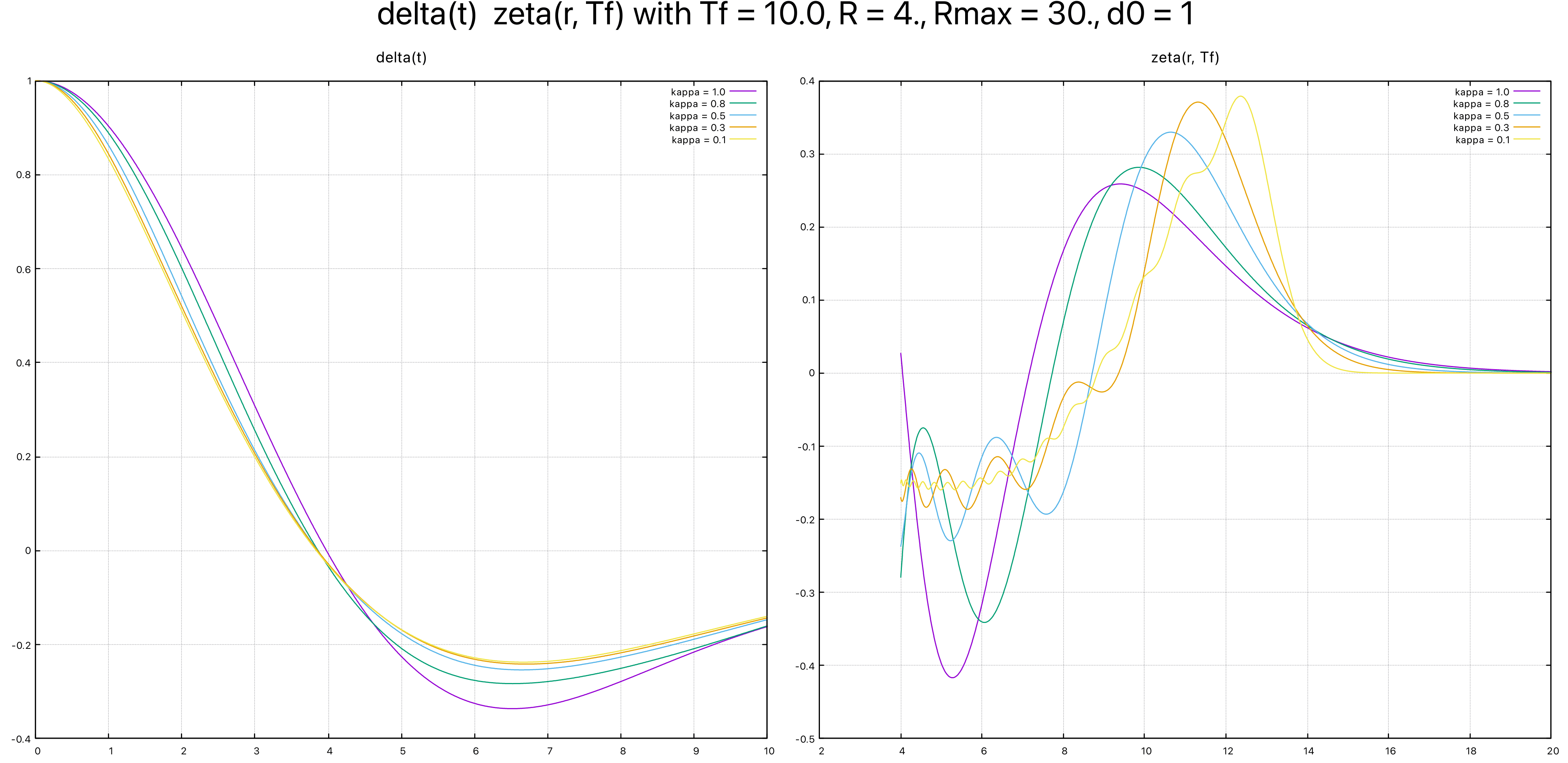
Figure - Simulations with different values of $\kappa$
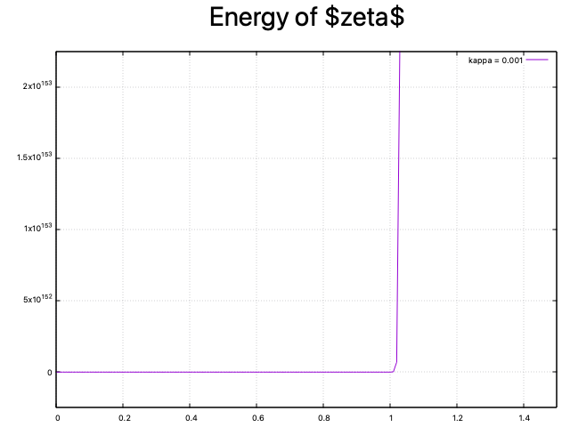
Figure - Simulations with $\kappa = 0.001$
$$
\left\{\begin{matrix}
\kappa^2 \ddot{\zeta} + \zeta = \mathcal{R} \zeta - \frac{R}{2}M^{-1} (\underline{\mathcal{R} \zeta} - \delta) G(r/\kappa), \\
M\ddot{\delta} + \delta = \underline{\mathcal{R}\zeta}.
\end{matrix}\right.
$$
The Fourier cos transform applied to the equation of $\zeta$:
$$
\forall k \in \mathbb{N}, \, \kappa^2 \ddot{\widehat{\zeta}_k} + \kappa^2 \omega_k^2 \widehat{\zeta}_k = c\kappa^2(\underline{\mathcal{R} \zeta} - \delta) \frac{1}{1+\kappa^2 k^2}, \quad \omega_k^2 = \frac{k^2}{1+\kappa^2 k^2}
$$
$\Rightarrow$ expression of $\widehat{\zeta}_k$ for all $k$,
Also $\forall u, \underline{\mathcal{R}u} = \int_0^{+\infty} \frac{\widehat{u}(k)}{1+\kappa^2k^2}dk$,
$\Rightarrow$ expression of $\underline{\mathcal{R}\zeta}$ for all $t$ as
$$
\forall t > 0, \, \underline{\mathcal{R}\zeta} = \underline{\mathcal{R}\zeta}^{\rm homog} + \int_0^t K(s-t)(\underline{\mathcal{R} \zeta}(s) - \delta(s))ds
$$
Discretization:
$$
\forall k \in \mathbb{N}, \,
\left\{\begin{matrix}
\widehat{\zeta}^{n+1}_k = \cos(\omega_k\Delta t) \widehat{\zeta}_k^{n} + \frac{\sin(\omega_k\Delta t)}{\omega_k}\widehat{\dot{\zeta}}_k^{n} + \frac{c}{1+\kappa^2 k^2} (\underline{\mathcal{R} \zeta}^n - \delta^n) \frac{1 - \cos(\omega_k\Delta t)}{\omega_k^2},
\\
\widehat{\dot{\zeta}}_k^{n+1}
= -\omega_k\sin(\omega_k\Delta t) \widehat{\zeta}_k^{n} + \cos(\omega_k\Delta t)\widehat{\dot{\zeta}}_k^{n} - \frac{c}{1+\kappa^2 k^2} (\underline{\mathcal{R} \zeta}^n - \delta^n)\frac{\sin(\omega_k\Delta t)}{\omega_k}.
\end{matrix}\right.
$$
\begin{equation}
\left\{\begin{matrix}
\delta^{n+1} = \cos(\Delta t \sqrt{M})\delta^{n} + \frac{\sin(\sqrt{M}\Delta t)}{\sqrt{M}}\dot{\delta}^{n} + (1 - \cos(\sqrt{M}\Delta t))\underline{\mathcal{R} \zeta}^n,\\
\dot{\delta}^{n+1} = -\sqrt{M}\sin(\sqrt{M}\Delta t) \delta^{n} + \cos(\sqrt{M}\Delta t)\dot{\delta}^{n} + \sin(\sqrt{M}\Delta t)\underline{\mathcal{R} \zeta}^n
\end{matrix}\right.
\end{equation}
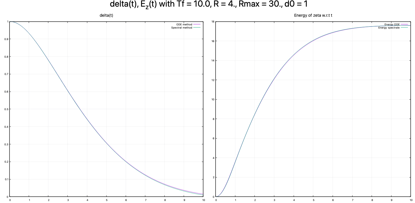
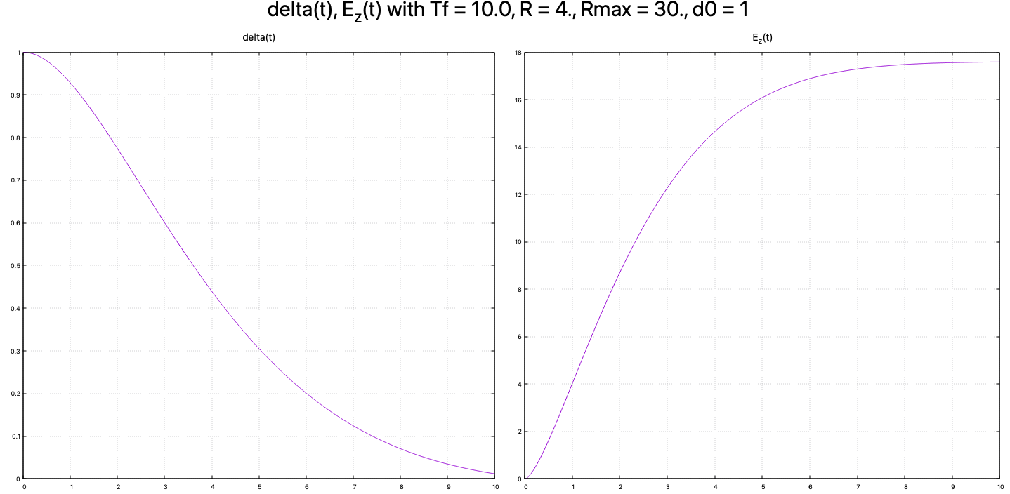
Figure - Comparaison of the methods with $\kappa = 0.3$
Figure - Spectral method with $\kappa = 10^{-5}$
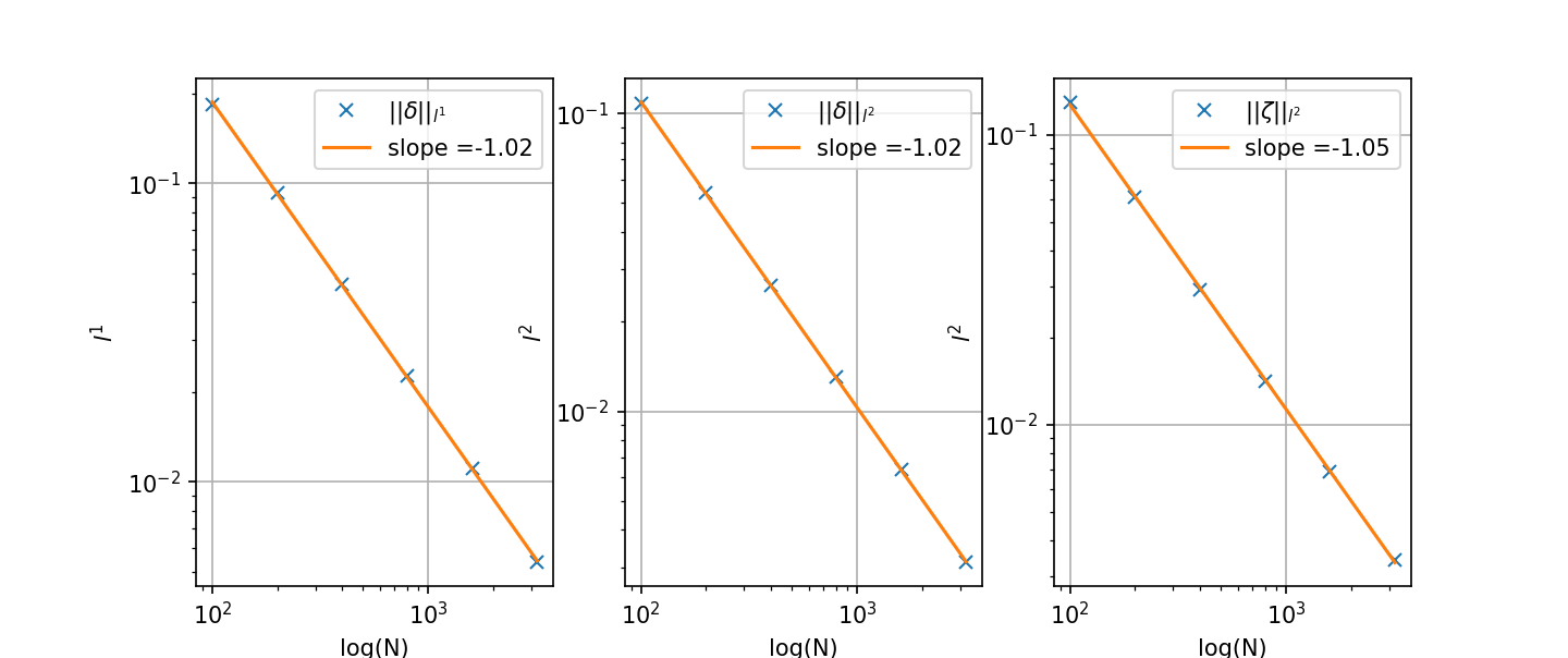
Convergence curve of the ODE computation to the raffined Spectral scheme, on $||\delta_{\rm EDO} - \delta_{\rm spec}||_{l^1_{\Delta t}}, ||\delta_{\rm EDO} - \delta_{\rm spec}||_{l^2_{\Delta t}}, ||\zeta_{\rm EDO} - \zeta_{\rm spec}||_{l^2_{\Delta x}}$.
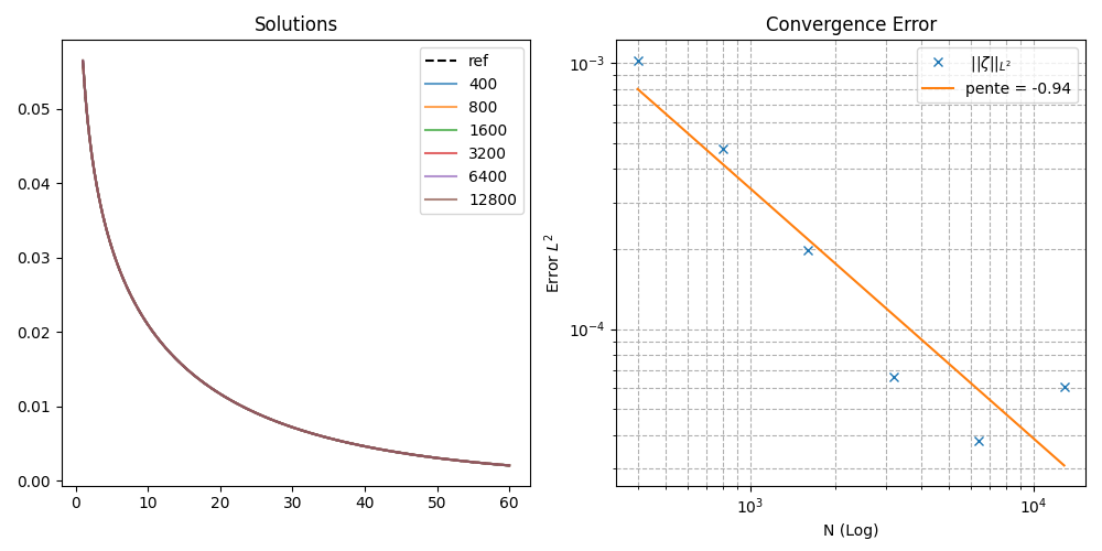
Convergence curve of $\zeta$ in the case where $\delta$ is given by $t\mapsto e^{-t/\tau}$, $\tau > 0$ a given parameter, and $\zeta$ has an exact solution.
Non-linear regime,
Flux scheme,
2D spectral method.
Thank you!
Slides created using reveal.js